CO2 Impact of Heat Pumps

Introduction

25.2 % of Germany’s energy budget are used for heating buildings, the majority of which (17.5 % points) is in the residential sector. As such, it produces immense emissions, $126 Mt$ in 2019 for example Bundesministerium für Wirtschaft und Klimaschutz. Reducing these emissions is of utmost importance to achieve the climate goals and mitigate the impact of global warming.

With the expansion of renewable electricity sources, heat pumps have the potential to provide a completely $CO_2$ neutral way of heating, but even with today’s electric mix, they usually produce less emissions than fossil based heat sources. In this project we built an tool analysis tool for researchers and end consumers to estimate their heating needs and the $CO_2$ impact of air-water heat pumps for residential buildings. The dashboard is available here.

Model Description

We model the building as an open thermodynamic system in a heat bath (outside environment). The entire building is assigned a single temperature, so like a homogeneous block in a perfectly equilibrated steady state. The building is parametrized by its heat capacity $C$, volume $V$, the specific heat transfer coefficients of its different surfaces $U_i$, the surface area of walls $A_{walls}$, roof $A_{roof}$, floor $A_{floor}$ and lastly windows $A_{windows}$. Specific heat capacities were taken from this paper on the role of specific heat capacity on building energy performance and thermal discomfort and interpolated manually for different building ages. The specific U values mapped to building age, according to the classes specified in Gebäudeenergiegesetz (GEG), Anlage 1. If solar radiation is simulated, the windows are assigned a value $g_{window}$ depending on the building age, which specifies the transmittance of vertical radiation through glass. This is lower for more modern, multi layer windows and higher for older, single layer windows Richtwerte finden sich in DIN 4108-4 als Gesamtenergiedurchlassgrade bei senkrechtem Strahlungseinfall. All the surface areas are computed from the living area input by the user, evenly split among the given number of floors by assuming $3 m$ height per floor and a flat, square roof and base of the building.

The transfer due to the temperature gradient to the outside at a given timestep is then:

$$\begin{equation} \dot{Q}=UA\Delta T = \sum{U_{i} A_{i} (T_{outside} - T_{house})} \end{equation}$$

This equation gets additional terms for ventilation, heat produced by electrical appliances, habitants, and heating due to solar radiation.

$$\begin{equation} \dot{Q}=UA(T_{outside} - T_{house}) + 0.95\cdot P_{internal} + g_{window} P_{solar} + P_{heat : pump} + n_{ventilation:rate} c_{air} V_{air} \rho_{air} \end{equation}$$

Finally, the temperature in the house is defined as $T_{house} = \frac{Q}{C}$. The resulting ODE is integrated with an explicit Euler integrator with a step size of $1 h$, which is the time resolution at which we handle all the data.

If “close window blinds in summer” is in the model assumptions, we redefine P*solar slightly, such that less solar radiation comes through the windows on hot days:

$$\begin{equation} P_{\text{solar:adjusted}} = \begin{cases} P_{\text{solar}} & \text{if } T_{\text{outside}} \le 22^\circ \text{C} \ 0.1 \cdot P_{\text{solar}} & \text{else} \end{cases} \end{equation}$$

Dashboard Overview

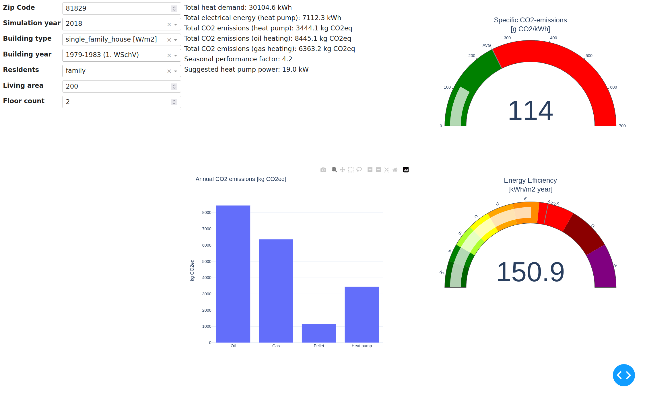
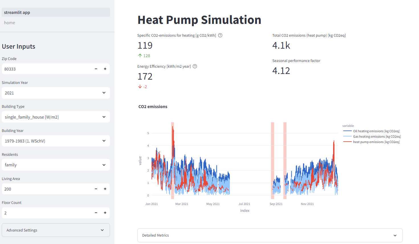
Simplified

The simplified model is populated by a series of sensible defaults for all inputs, which are not exposed to the user. For example, we set the $A_{windows}$ to 20 % of the living area, activate all available model assumptions except for weather forecast uncertainty and set the simulation range from 1. January to 31. December of the selected year. Based on $W/m^2$ heating requirement values from DIN EN 12831-1 we filter the available list of heat pump models and select a suitably sized pump automatically. By default the electricity mix is the German, historic electricity generation mix of the selected year, as downloaded from SMARD, a service offered by the Bundesnetzagentur. If no electricity data is available for the selected year, we repeat the closest available year periodically to fill the entire timeseries.

Academic

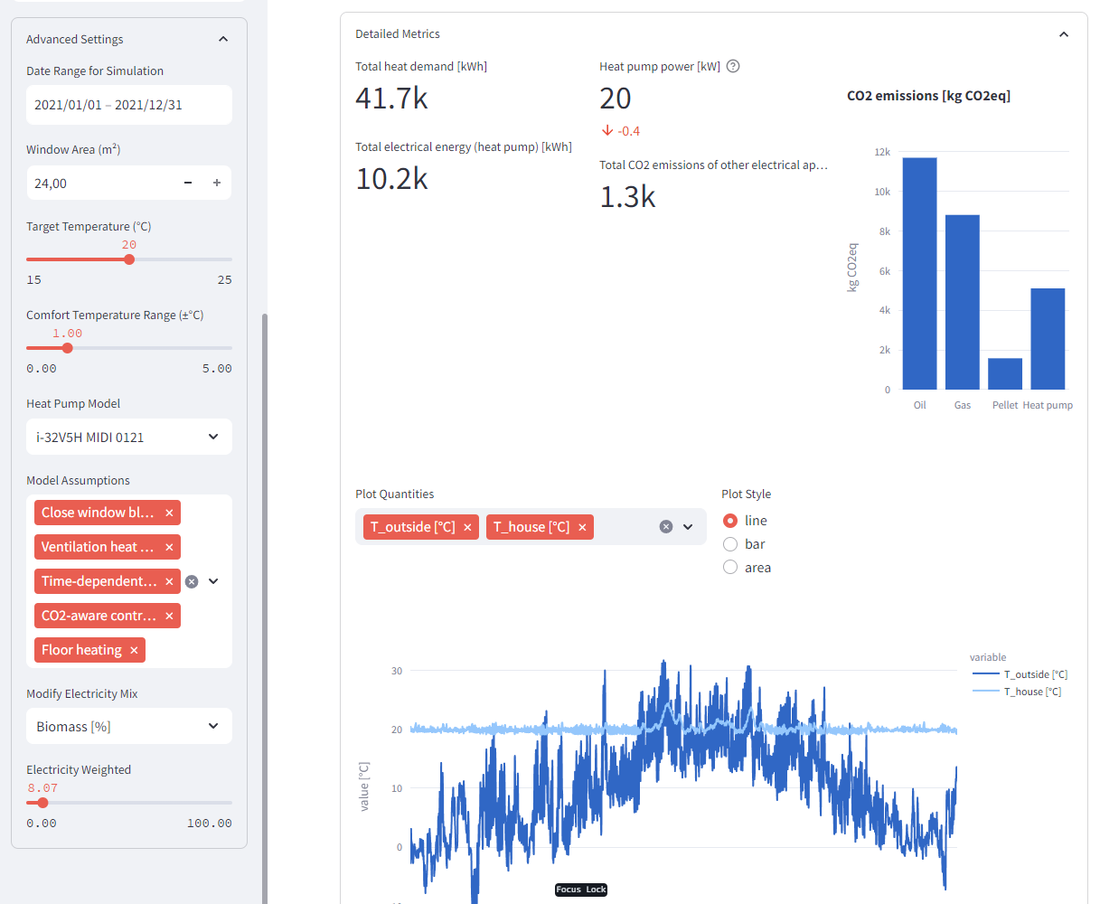
The academic Dashboard version is intended for deeper exploration of the data. We tried to expose as much control over the simulation parameters as possible, including some model assumptions. Particularly the electricity mix input is valuable for testing hypothetical scenarios, e.g. different expansions of renewable energies in as part of the energy mix. 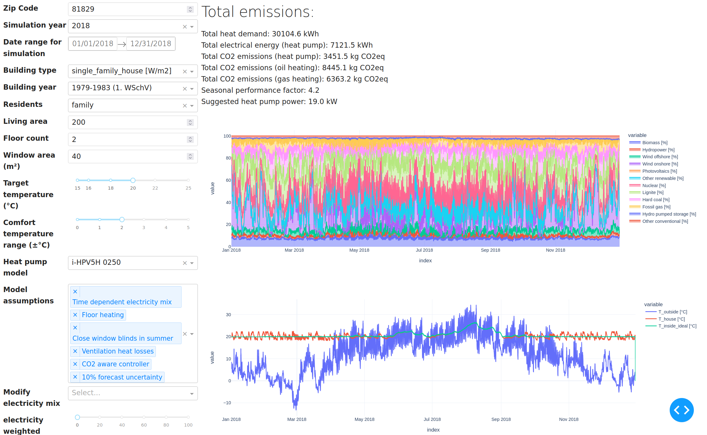The academic dashboard has customizable plots where the user can select arbitrary timeseries data to display. We tried to make all intermediate calculation steps available. The units are always marked in square brackets after the variable name and are automatically displayed on the y-axis label in the new dashboard version. Selecting the bar display type sums up the values in bins over the individual months, e.g. to analyze the monthly electricity usage. Since we are using $1 h$ timesteps and units of $kW$ where sensible, the aggregated bars conveniently show the total monthly elecctricity usage in $kWh$. The area plot is mostly useful to show quantities, which have a cumulative meaning, e.g. the percentages of different electricity sources in the current mix.

Column	Unit	Description
p_solar (south/east/west)	$kW/m^2$	Specific solar radiation strength for a vertical surface facing south/west/east respectively. This already includes corrective factors from literature for average shading, non-perpendicular radiation and self shadowing due to the window frame.
P_solar	$kW$	Total heating power due to solar irradiation, assuming equal distribution of windows over north, south, east and west. Computed as $\sum{A_{windows : i} \cdot p_{solar : i}}$
T_{outside}	$C^\circ$	Outside air temperature used for computing the heat losses and COP of the heat pump
T_{house}	$C^\circ$	Average temperature of the building. Air temperature and wall temperature are not treated independently.
Wind offshore, Biomass, Nuclear…	%	Percentage of the specific energy source in the electricity mix.
Intensity	$g\cdot CO_{2} {eqivalent}/kWh$	The $CO_2$ equivalent intensity of one $kWh$ electricity at the current timestep, computed by multiplying the fractions of different electricity sources with their specific $CO_2$ intensities
Intensity per heat	$g\cdot CO_{2} {eqivalent}/kWh$	The $CO_2$ equivalent intensity of one $kWh$ of heating using the heat pump, computed as $\frac{Intensity : electricity}{COP}$
P_el appliances	$kW$	Electricity consumption of household appliances, e.g. oven, computer… This is added to the house as heat using a factor of $0.95$
P_el heat pump	$kW$	Electricity consumption of the heat pump. This is not added as heat to the building.
Q_dot_demand	$kW$	Theoretical heat demand to fulfil the temperature requirements.
Q_dot_supplied	$kW$	Actual amount of heat supplied to the building by the heat pump. May be less than Q_dot_demand if the heat pump is chosen too small
Q_dot_transferred	$kW$	Heat transfer to the outside of the building through walls, windows, ceiling and floor.
Q_dot_ventilation	$kW$	Heat transfer due to periodic ventilation of the building. We assume that 35 % of the air volume in the building are replaced per hour (According to Standard 62.2-2016 - Ventilation and Acceptable Indoor Air Quality in Residential Buildings).

$CO_2$ controller

The controller tries to minimize $CO_2$ emissions, by heating when electricity is less $CO_2$ intensive. It is based on the single household model, described in Paper but was extended to use a variable optimization period. Initially we thought the metric to optimize for was g CO2eq/kWh of the current electricity mix, but we soon realized, that the temperature dependent COP of the heat pump also has to be taken into consideration. We actually want to heat when g CO2eq/kWh heating is minimal. This metric takes into account both the temperature dependent COP and the $CO_2$ intensity of the electricity mix.

Initially we used time window of $48 h$ for computation. We estimate the heat demand during that time interval based on a temperature and usage forecast, which we simulate by adding 10 % uniform random noise to the true temperature and usage profiles. Using a fixed time window of $48 h$ the controller produced strong temperature oscillations in the winter, since in extreme cases it would heat for a day (e.g. a windy day, when the electricity is clean) and turn off the other day. In old buildings with poor isolation, this caused temperature deviations of up to $\pm 4 ^\circ C$ from the target temperature, since the cooling rate was simply too high to allow for such a long heating pause.

We therefore introduced an extension to the base control strategy, that allows to choose a minimum and maximum temperature, from which a time window for optimization is computed. The window is simply determined by the time it takes for the building to get colder or hotter than the minimum temperature naturally. Thereby we ensure, that even in the most extreme cases (no heating for the entire period) the temperature deviation is limited. The controller is now able to produce a much more stable temperature profile, while still optimizing for $CO_2$ emissions. An added benefit is, that it can now also use longer periods for optimization if the house has a sufficient heat capacity to isolation ratio or when the outside temperature is close to target temperature anyway.

Of course a larger temperature variation allows for lower $CO_2$ emissions, since the controller has more freedom to choose when to heat, as can be seen in the following figure. Note that allowing a larger temperature variation does not change the average temperature in the building. 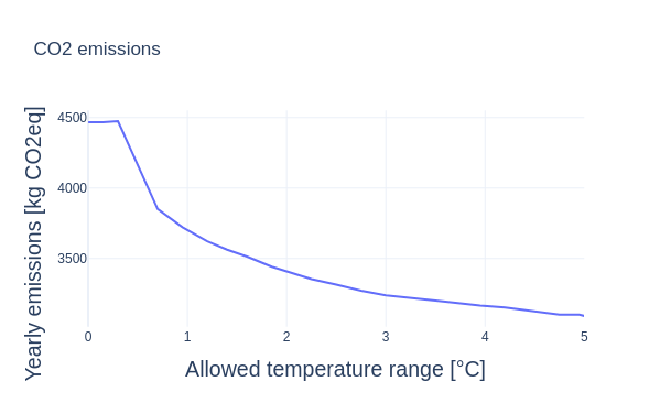All the figures in this section are computed for a $200 m^2$ building from 1980, with the reference usage profile set to family and simulation year 2021.

Model validation and results

To validate our model, we compared the results to various rule of thumb formulas from DIN-12831.

There are tabular reference values for the maximum outside temperature at which heating is required (Heizgrenztemperatur) defined in the standard. Since real buildings have a significant heat capacity, they react delayed to temperature changes. We therefore read off the 7 day moving average of $T_{outside}$ at points when the heat pump turned off for more than 7 consecutive days. The results deviated by $\le 0.5^\circ C$ from the tabular values in all trsted buildings below KfW70. For modern buildings, our simulation predicted shorter heating periods than the standard.

We also compared our model to standard heating load profiles and got results within a reasonable deviation range of $\pm$ 10 %.

Finally we compared our results to a real single family house from 1980, for which we knew the heat demand in previous years. We also had estimated heat demands, heat capacities and specific transfer coefficients of the building as determined by a heating consultant. The heat capacity computed by the model is 22 % below our reference. The heat transfer estimate on the other hand is very close. Our model predicts $34600 kWh$ of heat demand in 2021 ($29700 kWh$ in 2020, due to a milder winter), compared to the $\approx 30000 kWh$ historically used for heating.

In general we noticed that our model predicted lower heat demand for modern KfW70, KfW40 and GEG20 buildings, compared to the DIN standard. We also observed excessive heating in the summer, due to solar radiation and other internal gains. This is apparently a known issue with the standard, as it completely ignores internal heat sources, even though they are a relevant factor in well isolated buildings.

Outlook and Conclusion

Take into account more factors, e.g. To further enhance our analysis, it is crucial to consider additional factors, such as the influence of domestic hot water consumption, which is likely to have a significant role in the overall system dynamics.

In addition, exploring the economic implications alongside environmental impacts presents an intriguing avenue. This can be achieved with minimal algorithmic adjustments, primarily involving the substitution of data sources. Although we briefly experimented with modeling a hot water storage tank within the household, it only resulted in minimal impact on the outcome. In reality, hot water storage tanks are essential for any heat pump installation, as they service the short bursts of domestic hot water demands, for which the heat pump would react too slowly.

Time dependent electricity mix played a smaller role than expected. Especially when using the $CO_2$ aware control strategy, the difference is very small. With an increasing flow temperature (disabled floor heating model assumption), the impact becomes more noticable. In those cases, doing the simulation with the average intensity would underestimate the $CO_2$ impact of heat pumps by up to 10 %

Appendix

Heat pump library

For accurate heat pump models we are using hplib

Citation: Tjarko Tjaden, Hauke Hoops, Kai Rösken. (2021). RE-Lab-Projects/hplib: heat pump library (v2.0). Zenodo. https://doi.org/10.5281/zenodo.5521597

Load profiles

Electric and hot water load profiles for different households were generated by Fraunhofer ISE. An additional dataset for hot drinking water was taken from the district energy planning tool nPro

Carbon intensity factors

We follow the methodology described by electricitymaps.com with most data aggregated from this 2014 IPCC report. Hydro pumped storage was adjusted for Germany, as the global estomate is too optimistic. According to the Department of Economics at the University of Verona the effective carbon footprint is 31 % above the grid average due to round trip losses. electricitymaps.com does not account for these additional losses. Additionally the $CO_2$ intensity of German electricity is above the global average, so Germany’s mean intensity should be used as the baseline instead.

Electricity stats for Germany

SMARD

Specific heat demand

• Heizlastberechnung Bosy
• Heizlastrechner Waermepumpe.de
• NPro Heizlast profiles
• Heating limit temperature

Values for the 1980 house we used for comparisons
Living area:	200 $m^2$
Window area:	51.9 $m^2$
Heat capacity:	328000 $\frac{kJ}{K}$
Average specific heat conductance:	0.7293 $\frac{W}{m^2 K}$
Air volume:	1251 $m^3$
Historic heating oil consumption:	3000 $l$
Historic heating power consumption:	30000 $kWh$