Ever since I started playing around with the 3D software Blender in high school, I was fascinated by light transport simulations. Especially ray tracing, often hailed as the gold standard in rendering, is the algorithm behind a lot of stunningly realistic images in movies, video games, and even scientific visualizations. And what better way to learn about their inner workings than to implement one yourself? So I rolled up my virtual sleeves and embarked on a guided journey with Peter Shirley’s excellent book series Ray Tracing in One Weekend.
What is Ray tracing
In its essence, a ray tracer mimics the behavior of light rays as they travel through the world, just in reverse. Imagine you’re standing in a virtual world, surrounded by objects. To create an image of this scene, the ray tracer shoots rays from your viewpoint (the camera) into the scene. These rays bounce around, interacting with objects, and eventually reach a light source. Along the way, they gather information about the color, texture, and lighting of the objects they encounter. This process is repeated for every pixel in the image, resulting in a photo realistic representation of the scene.

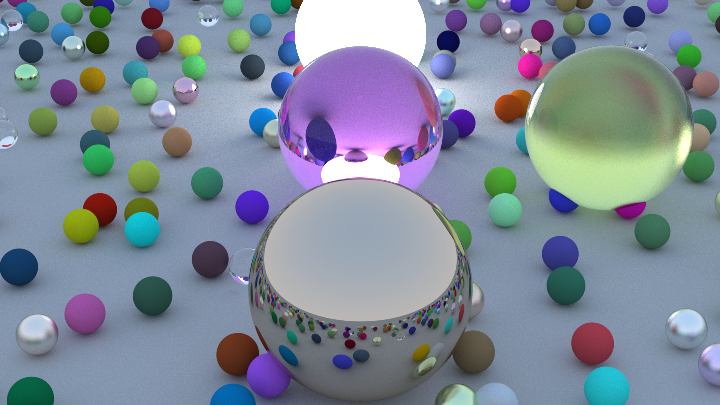
Reference image of 3 spheres made from different materials
After finishing the base ray tracer, which includes sphere, cube and triangle as the shape primitives with diffuse, specular, metal for the materials, I wanted to get more realistic.

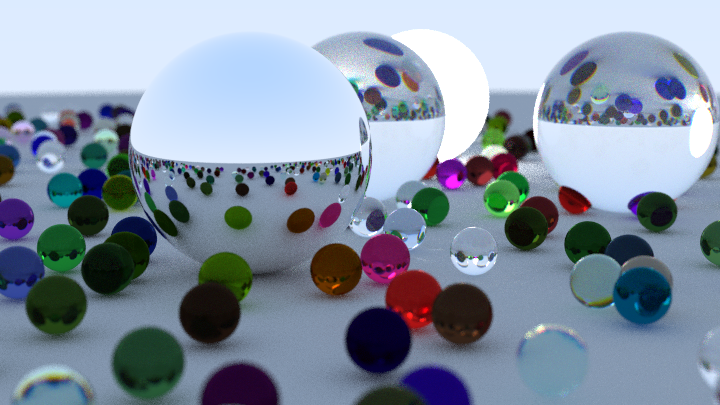
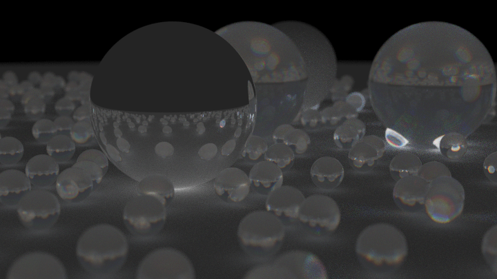
Programmatically generated scene with concentric glass spheres.
Dispersion
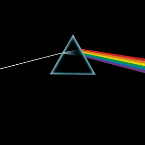
Ever since Pink Floyd invented prisms in their iconic publication “The Dark Side of the Moon”, humans were fascinated by dispersion and the pretty lights it produces.
Dispersion means that different wavelengths of light bend by varying degrees, when passing through a medium. The dispersion relation is a material specific property, and not all exhibit it to the same degree (that’s why diamons sparkle in so many colors and glass shards do not). To simulate it correctly, I needed to include spectral information in the rendering. Each traced ray now also has a wavelength associated with it, which is used when computing the dispersion and converted back to a color when writing the pixel.
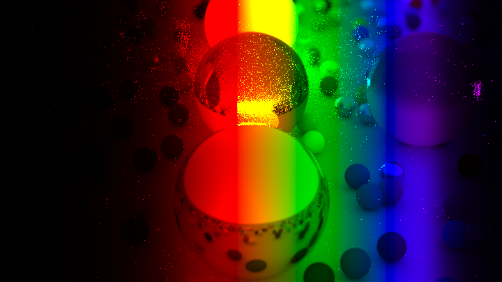
Dispersion is visible at the edges of the glass spheres (rainbow colored edges)
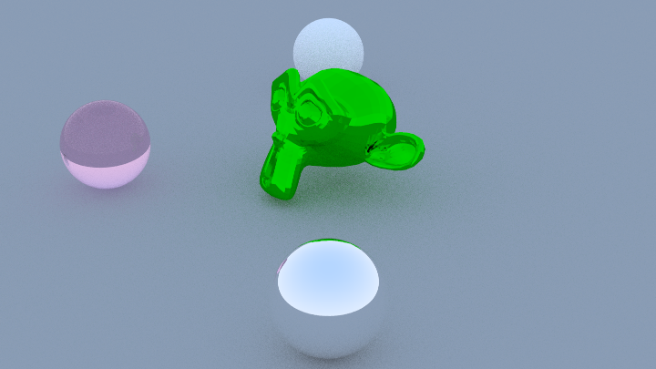
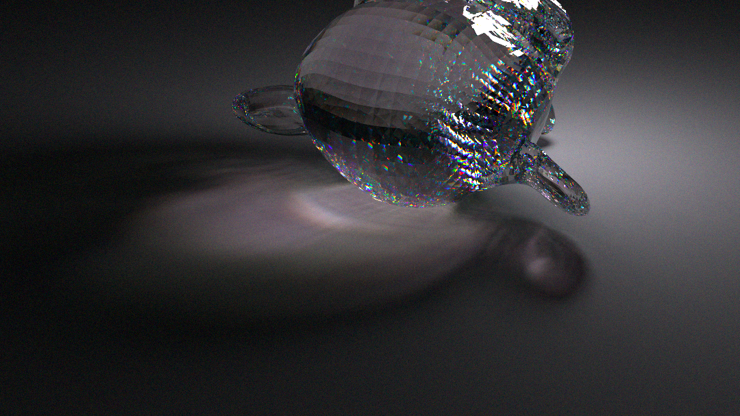 Caustics and dispersion from a sphere light through a triangle mesh.
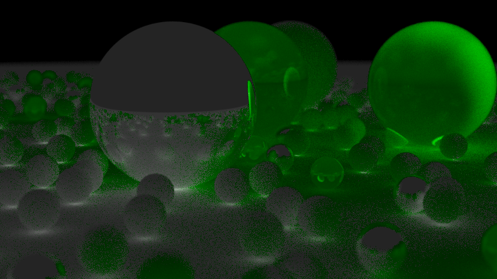
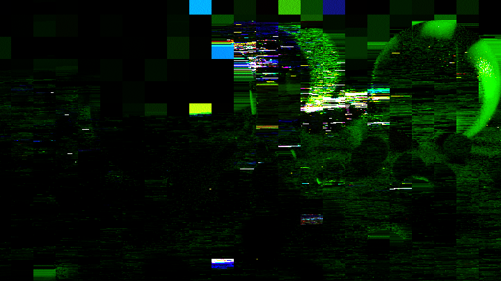
The inclusion of spectral information immediately makes the rendering much slower, since we now don’t just need one ray to estimate the color of a point, but have to average over many wavelengths instead. Since this is just unnecessary work when no dispersion is present, I added an optimization. Rays start out with color information, and only switch to a spectral representation when dispersed (i.e. they pass through glass). In reality, all materials have some sort of dispersion relation, but the ray tracer only simulates it for dielectric materials, where it is most noticeable. Coloring all light rays that traveled through glass in green for debugging purposes produces the following image (green pixels rays were split into multiple wavelengths and are hence significantly more expensive to calculate. Debug image is the same scene as above).
Black-body Radiation
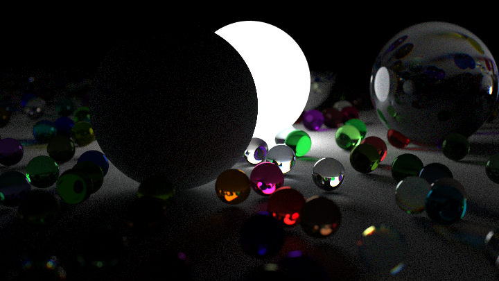
This also means, that the light sources suddenly don’t just need a color, but an emission spectrum as well! Any hot body (like the sun, or a classical light bulb) will approximately emit a so-called black body spectrum, due to the motion of its atoms. By sampling our wavelengths from this distribution, we can realistically simulate the color of black body radiation at different temperatures!

2000K blackbody radiation

4500K blackbody radiation

8000K black body radiation

Image produced by changing the temperature of the light source during the render
Per-Pixel Variance Estimation
By implementing per-pixel variance estimation, I introduced an optimization that significantly speeds up rendering while maintaining visual quality. This technique allows the renderer to exit early if the noise in a pixel falls below a certain threshold, focusing computational resources where they’re most needed.

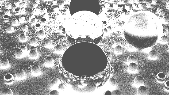
These three images show the effect of adaptive sampling. The first image is rendered with a constant number of samples per pixel and the second with adaptive sampling. Although the second image has the same total numer of samples as the first one, it has less visible noise (especially on the diffuse areas around the light and in shadows). The third image (black and white) shows which areas were sampled more often. The adaptive sampling algorithm estimates the variance of each pixel at runtime and decides whether to continue sampling or not.
Gallery
Rainbow produces by interpolating RGB looks unnatural and would not produce realistic dispersion.

Rainbow produced by simulating the intensity of different wavelengths using the planck spectrum. The wavelengths are convoluted by the sensitivity spectrum of our eyes receptors to get the color we would see. This produces a realistic spectrum image and much better dispersion.
Artifacts caused by race conditions between multiple threads which try to write into the image array.
Testing OBJ file loading
Simplified RGB dispersion model, debug image
What happens if we apply a cross product instead of a dot product to the normals?
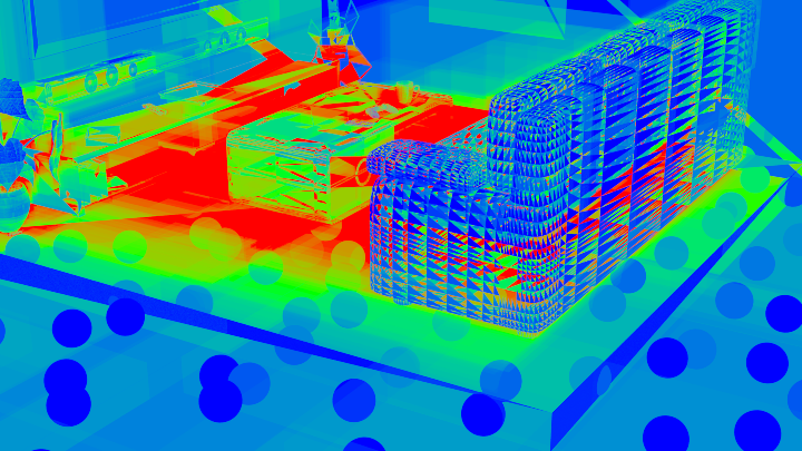
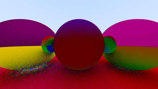
Debug view showing the BVH traversal cost, when splitting on the longest axis. Red is expensive, blue is cheap.